Getting started with yieldplotlib#
Introduction#
This tutorial will walk you through some of the basic functionality of yieldplotlib to get you started on generating your own yield visualizations.
yieldplotlib is designed to standardize outputs from different mission simulation tools (currently AYO and EXOSIMS) into a single, unified format. This allows you to write a plotting script once and apply it to results from entirely different yield calculators without changing your code and it facilitates easy comparisons between the tools.
To run yieldplotlib you need to have at least one AYO output folder, EXOSIMS output folder, or yield input package (YIP). Sample data has been provided in the tutorials folder of this repository for demonstrative purposes. You can also run series of pre-made plots for yield outputs which can be found in the yieldplotlib/src/scripts folder, or accessed through the yieldplotlib pipeline and command line interface.
Imports#
import logging
import matplotlib.pyplot as plt
from IPython.display import HTML
import yieldplotlib as ypl
from yieldplotlib.accessibility import AccessibilityManager
from yieldplotlib.logger import logger
from yieldplotlib.plots.yip_plots import make_offax_psf_movie, plot_core_throughtput
/home/docs/checkouts/readthedocs.org/user_builds/yieldplotlib/envs/latest/lib/python3.12/site-packages/tqdm/auto.py:21: TqdmWarning: IProgress not found. Please update jupyter and ipywidgets. See https://ipywidgets.readthedocs.io/en/stable/user_install.html
from .autonotebook import tqdm as notebook_tqdm
Loading Yield Data#
We can load our sample AYO and EXOSIMS data using the AYODirectory and EXOSIMSDirectory classes. These classes parse the output directories and prepare them for querying.
%%capture
logger.setLevel(logging.ERROR)
# Load the sample data provided in the GitHub repository
ayo = ypl.fetch_ayo_data()
exosims = ypl.fetch_exosims_data()
# Normally this looks more like this:
# ayo_folder = Path("sample_data/ayo")
# exosims_folder = Path("sample_data/exosims")
# ayo = AYODirectory(ayo_folder)
# exosims = EXOSIMSDirectory(exosims_folder)
Downloading file 'ayo.zip' from 'https://github.com/HWO-Yield-Visualizations/yieldplotlib/raw/main/data/ayo.zip' to '/home/docs/.cache/yieldplotlib'.
Unzipping contents of '/home/docs/.cache/yieldplotlib/ayo.zip' to '/home/docs/.cache/yieldplotlib/ayo.zip.unzip'
Downloading file 'exosims.zip' from 'https://github.com/HWO-Yield-Visualizations/yieldplotlib/raw/main/data/exosims.zip' to '/home/docs/.cache/yieldplotlib'.
Unzipping contents of '/home/docs/.cache/yieldplotlib/exosims.zip' to '/home/docs/.cache/yieldplotlib/exosims.zip.unzip'
Now that we have loaded our directories, we can display the file structure to see what is contained in our yield outputs at a glance.
logger.setLevel(logging.WARNING)
print(exosims.display_tree())
print(ayo.display_tree())
<EXOSIMSDirectory: exosims>
├── <DRMDirectory: drm>
│ ├── <DRMFile: 602765987.pkl>
│ ├── <DRMFile: 297122009.pkl>
│ ├── <DRMFile: 785267868.pkl>
│ ├── <DRMFile: 611229025.pkl>
│ ├── <DRMFile: 268142898.pkl>
│ └── ... and 95 more
├── <EXOSIMSCSVDirectory: csv>
│ ├── <EXOSIMSCSVFile: reduce-times.csv>
│ ├── <EXOSIMSCSVFile: reduce-info.csv>
│ ├── <EXOSIMSCSVFile: reduce-earth-char-count.csv>
│ ├── <EXOSIMSCSVFile: reduce-promote-hist.csv>
│ ├── <EXOSIMSCSVFile: reduce-radlum.csv>
│ └── ... and 12 more
├── <SPCDirectory: spc>
│ ├── <SPCFile: 602765987.spc>
│ ├── <SPCFile: 963082196.spc>
│ ├── <SPCFile: 668276647.spc>
│ ├── <SPCFile: 911031869.spc>
│ ├── <SPCFile: 969890527.spc>
│ └── ... and 95 more
└── <EXOSIMSInputFile: Example_EXOSIMS.json>
<AYODirectory: ayo>
├── <AYOCSVFile: observations.csv>
├── <AYOCSVFile: coronagraph1.csv>
├── <AYOInputFile: yield_run.ayo>
└── <AYOCSVFile: target_list.csv>
The Common Parameter Interface#
A core feature of yieldplotlib is the standardized set of “Common Parameters” that can be accessed. These parameters pull the same data from different yield codes without requiring a user to parse the underlying files and keys themself.
The interactive table below lists the currently supported parameters available for querying. You can use the search box to filter by keyword (e.g., try typing “magnitude”, “yield”, or “coronagraph”) to find the specific key you need for your plots.
Note: For a static version of this table see the Common Parameters documentation page. To learn more about how this works see Parsing and Getting Values.
import io
import pandas as pd
from itables import show
def read_markdown_table(filepath):
"""Parses our markdown table file into a Pandas DataFrame."""
with open(filepath) as f:
lines = f.readlines()
clean_lines = [line for line in lines if "|" in line and "---" not in line]
clean_data = "".join(clean_lines)
df = pd.read_csv(io.StringIO(clean_data), sep="|", engine="python")
df = df.dropna(axis=1, how="all")
df.columns = [c.strip() for c in df.columns]
df = df.apply(lambda x: x.str.strip() if x.dtype == "object" else x)
return df
df_params = read_markdown_table("../user/parameters_table.md")
show(df_params, classes="display", paging=True, pageLength=10)
| Loading ITables v2.8.0 from the internet... (need help?) |
Accessing Data and Generating Plots#
We have our data loaded and can now start accessing it and generating plots!
Get Data#
Data can be accessed from the AYODirectory and EXOSIMSDirectory using the .get() function which takes the named yieldplotlib keys as input and outputs the corresponding values. This can be in the form of singular values or arrays.
# Pupil diameter
ayo_pup = ayo.get("pupil_diam")
exo_pup = exosims.get("pupil_diam")
print(f"Pupil diameters are:\nAYO: {ayo_pup} \nEXOSIMS: {exo_pup}")
# ExoEarth yields
ayo_yield = ayo.get("yield_earth")
exo_yield = exosims.get("yield_earth")
print(f"\nExoEarth yields are:\nAYO: {ayo_yield} \nEXOSIMS: {exo_yield}")
# Target star distances (first 10)
ayo_dist = ayo.get("star_dist")
exo_dist = exosims.get("star_dist")
print(f"\nStellar distances (pc) are:\nAYO: {ayo_dist[:10]} \nEXOSIMS: {exo_dist[:10]}")
Pupil diameters are:
AYO: 7.22577 m
EXOSIMS: 7.225765
ExoEarth yields are:
AYO: 21.81181898211
EXOSIMS: [17.15]
Stellar distances (pc) are:
AYO: [ 1.34749 3.49736 1.34749 5.12952 7.70357 7.4783 11.3417 11.091
15.3728 13.9204 ] pc
EXOSIMS: [26.39 15.89 4.34 11.31 25.71 13.67 27.44 18.75 21.28 20.19] pc
Generic Plots#
yieldplotlib expands directly on matplotlib to utilize its functionality and to make plot customization intuitive for those who have familiarity with matplotlib and its features. Below are examples of some of the generic yieldplotlib plots that one can make.
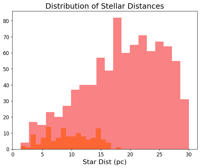
# Histograms
fig, ax = plt.subplots(figsize=(8, 6))
ax.ypl_hist(exosims, x="star_dist", bins=20, alpha=0.7, label="EXOSIMS Stars")
ax.ypl_hist(ayo, x="star_dist", bins=20, alpha=0.7, label="AYO Stars")
ax.set_title("Distribution of Stellar Distances")
plt.show()
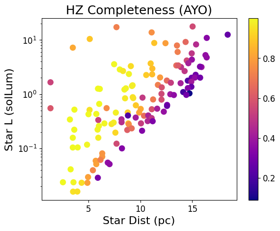
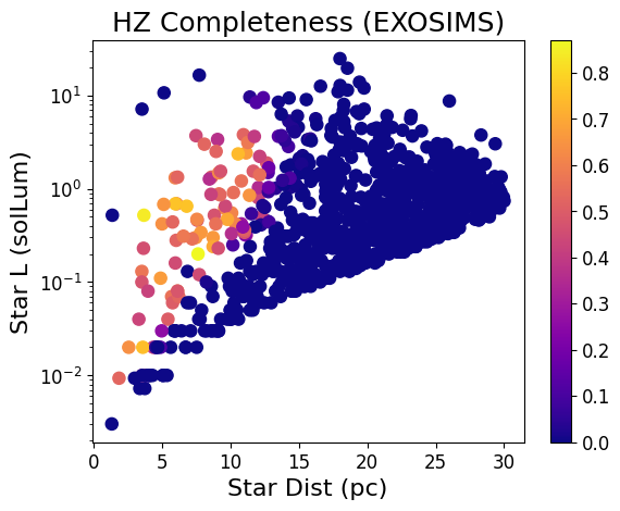
# Scatter Plots
fig, ax = plt.subplots()
data = ax.ypl_scatter(ayo, x="star_dist", y="star_L", c="star_comp_det")
ax.set_title("HZ Completeness (AYO)")
ax.set_yscale("log")
plt.colorbar(data)
fig, ax = plt.subplots()
data = ax.ypl_scatter(exosims, x="star_dist", y="star_L", c="star_comp_det")
ax.set_title("HZ Completeness (EXOSIMS)")
ax.set_yscale("log")
plt.colorbar(data)
plt.show()
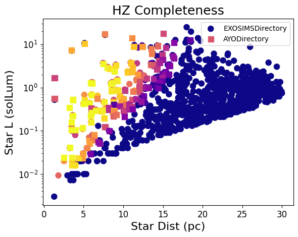
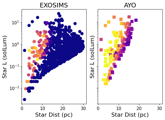
Comparative Plots#
Instead of plotting datasets individually, for comparison purposes it is often desired to plot different yield outputs in a single figure. Here the suite of available yieldplotlib comparative plots should be used. Lets see two examples plotting the same HZ completeness plot as above.
# Two yield runs on same set of axes.
fig, ax = plt.subplots()
ax.set_title("HZ Completeness")
data = ypl.compare(
ax,
[exosims, ayo],
x="star_dist",
y="star_L",
plot_type="scatter",
c="star_comp_det",
)
ax.set_yscale("log")
plt.show()
# Two yield runs on different sets of axes.
fig, axs = ypl.multi(
[exosims, ayo],
x="star_dist",
y="star_L",
plot_type="scatter",
c="star_comp_det",
sharex=True,
sharey=True,
titles=["EXOSIMS", "AYO"],
)
axs[0, 0].set_yscale("log")
plt.show()
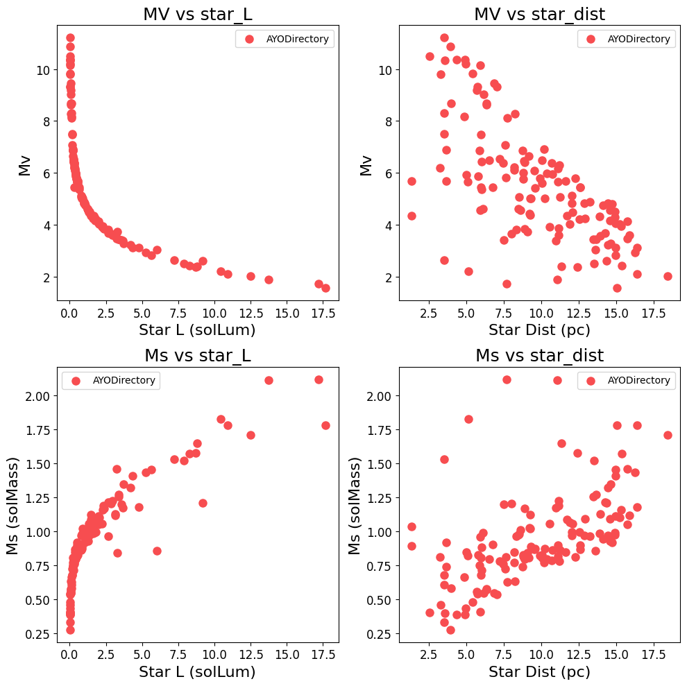
Additionally, we can run more complex analyses on multi-dimensional grids of parameter space.
# Plot a grid of parameters against each other.
fig, axs = ypl.xy_grid(
[ayo],
["star_L", "star_dist"],
["MV", "Ms"],
plot_type="scatter",
legend=True,
)
plt.show()
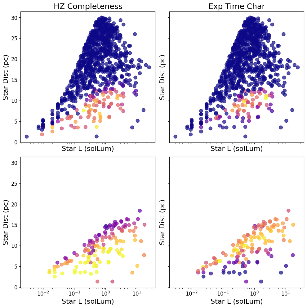
# Plot multiple panels with different specifications for each yield run.
spec1 = {
"x": "star_L",
"y": "star_dist",
"plot_type": "scatter",
"c": "star_comp_det",
"alpha": 0.7,
}
spec2 = {
"x": "star_L",
"y": "star_dist",
"plot_type": "scatter",
"c": "exp_time_char",
"alpha": 0.7,
}
specs = [spec1, spec2]
fig, axes = ypl.panel(
[exosims, ayo],
*specs,
figsize=(10, 10),
suptitle=None,
layout=None,
sharex=True,
sharey=True,
titles=["HZ Completeness", "Exp Time Char", "", ""],
)
axes[1, 0].set_xscale("log")
plt.show()
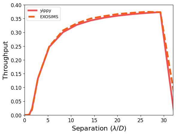
Yield Input Package (YIP) Loading#
yieldplotlib supports the loading and plotting of yield input packages using yippy as a back end. YIPs specify relevant coronagraph parameters for yield codes and so are often critical inputs to be able to vet and visualize.
# Load the YIP data
yip = ypl.fetch_yip_data()
# Normally looks like this
# yip_folder = Path("sample_data/yip")
# yip = YIPDirectory(yip_folder)
Downloading file 'yip.zip' from 'https://github.com/HWO-Yield-Visualizations/yieldplotlib/raw/main/data/yip.zip' to '/home/docs/.cache/yieldplotlib'.
Unzipping contents of '/home/docs/.cache/yieldplotlib/yip.zip' to '/home/docs/.cache/yieldplotlib/yip.zip.unzip'
Loading YIPDirectory yip: 0%| | 0/6 [00:00<?, ?item/s]
[yieldplotlib] WARNING [2026-05-25 23:30:15,174] Unknown file type:
Loading YIPDirectory yip: 100%|██████████| 6/6 [00:00<00:00, 805.13item/s]
[yieldplotlib] WARNING [2026-05-25 23:30:15,181] No input files found
[yippy] INFO [2026-05-25 23:30:15,182] Creating yip coronagraph
[yippy] WARNING [2026-05-25 23:30:15,184] Unhandled header fields: {'TMULDET', 'TMULCHAR'}
[yippy] WARNING [2026-05-25 23:30:15,185] Using default unit for D: m. Could not extract unit from comment: "circumscribed diameter of the telescope in mete"
[yippy] WARNING [2026-05-25 23:30:15,185] Using default unit for D_INSC: m. Could not extract unit from comment: "inscribed diameter of the telescope in meters"
[yippy] INFO [2026-05-25 23:30:15,236] yip is radially symmetric
[yippy] INFO [2026-05-25 23:30:15,460] No precomputed performance file found. Computing all performance metrics...
[yippy] INFO [2026-05-25 23:30:15,461] Computing throughput curve...
[yippy] INFO [2026-05-25 23:30:15,948] Computing raw contrast curve...
[yippy] INFO [2026-05-25 23:30:16,003] Computing core area curve...
[yippy] INFO [2026-05-25 23:30:16,036] Computing occulter transmission curve...
[yippy] INFO [2026-05-25 23:30:16,242] Computing core mean intensity curve...
[yippy] INFO [2026-05-25 23:30:16,441] OWA set to max_offset_in_image: 32.00 lam/D
[yippy] INFO [2026-05-25 23:30:16,442] Created yip
plot_core_throughtput(
[exosims], ["EXOSIMS"], yip=yip, ax_kwargs={"xlim": (0, 32), "ylim": (0, 0.4)}
)
[yippy] INFO [2026-05-25 23:30:16,454] Computing throughput curve...
[yippy] INFO [2026-05-25 23:30:17,215] Computing raw contrast curve...
[yippy] INFO [2026-05-25 23:30:17,263] Computing core area curve...
[yippy] INFO [2026-05-25 23:30:17,296] Computing occulter transmission curve...
[yippy] INFO [2026-05-25 23:30:17,299] Computing core mean intensity curve...
[yippy] INFO [2026-05-25 23:30:17,326] OWA set to max_offset_in_image: 32.00 lam/D
(<Figure size 640x480 with 1 Axes>,
<Axes: xlabel='Separation ($\\lambda/D$)', ylabel='Throughput'>)
# Make GIF animation of the off-axis stellar PSF.
ani = make_offax_psf_movie(yip, "offax_psf_animation.gif")
# Code to easily view the animation in the notebook.
HTML(ani.to_jshtml())
MovieWriter ffmpeg unavailable; using Pillow instead.